- ImageMagick
- Gnuplot online - BETA
- Docker Hub - jweissig/alpine-imagemagick
- GitHub - jweissig/alpine-imagemagick
- Docker Desktop
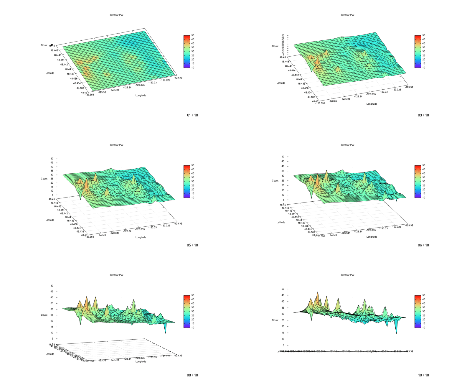
- Gnuplot images (10 images for gif)
In this episode, we are going to walk through an end-to-end workflow for creating animated GIFs using Docker and ImageMagick. I wanted to highlight this useful pattern for using utility containers on your desktop because it delivers very reproducible results.

Here is the animated GIF we will be creating today. I created this with Docker and ImageMagick and I wanted to show you my workflow for doing this today. If you have not used ImageMagick before, it is basically the swiss army knife of image manipulation at the command-line. Just an incredible tool and makes this type of stuff very easy.

So, why am I doing this? Well, in an upcoming episode, we will be collecting some sensor data, cleaning and exploring the data, then plotting the dataset on to a map. This was sort of a personal project have I been working on. I created these source images using this pretty cool site where it is an online version of Gnuplot.
Basically, you enter your data, this is my data here and I posted it in the episode notes below too. Just in case you want to try.
# X          Y         Z
-123.3224397    48.4411657  25
-123.3241633    48.4406032  29
-123.3254599    48.4415822  13
-123.3297772    48.4429775  22
-123.3405445    48.4380596  14
-123.3319104    48.4352701  62
-123.3237204    48.4365414  28
-123.3276267    48.4450817  6
-123.3414154    48.4405798  28
-123.3440098    48.4425372  69
-123.3345387    48.4484350  69
-123.3297604    48.4373741  62
-123.3383769    48.4345608  23
-123.3383948    48.4401639  25
-123.3349479    48.4412894  27
-123.3340947    48.4443726  40
-123.3483089    48.4383282  14
-123.3530528    48.4381807  4
-123.3396738    48.4355394  24
-123.3435650    48.4384754  21
-123.3254761    48.4471860  7
-123.3491608    48.4352452  41
-123.3422679    48.4374967  37
-123.3288904    48.4348539  31
-123.3517554    48.4372022  82
-123.3388212    48.4386223  42
-123.3470116    48.4373496  19
-123.3444360    48.4409956  39
-123.3422863    48.4431001  45
-123.3431388    48.4400169  18
-123.3228824    48.4452279  18
-123.3211431    48.4401867  21
-123.3328148    48.4489978  29
-123.3250331    48.4431237  31
-123.3258868    48.4400407  17
-123.3327977    48.4433937  25
-123.3366537    48.4351235  49
-123.3340774    48.4387691  56
-123.3284471    48.4307926  55
-123.3474568    48.4414113  74
-123.3444173    48.4353924  103
-123.3521813    48.4356607  37
-123.3371155    48.4447887  21
-123.3332243    48.4418521  44
-123.3233094    48.4436863  20
-123.3245901    48.4390617  21
-123.3215701    48.4386452  21
-123.3207006    48.4361249  2
-123.3319274    48.4408733  63
-123.3315008    48.4424148  31
-123.3211275    48.4345836  8
-123.3345213    48.4428310  20
-123.3526269    48.4397222  8
-123.3496062    48.4393067  73
-123.3336336    48.4347075  72
-123.3297436    48.4317713  36
-123.3439911    48.4369339  52
-123.3284637    48.4363952  41
-123.3370978    48.4391851  17
-123.3211586    48.4457904  18
-123.3314838    48.4368115  8
-123.3293170    48.4333126  8
-123.3250170    48.4375203  17
-123.3345039    48.4372276  49
-123.3392655    48.4426842  22
-123.3457333    48.4419743  80
-123.3461405    48.4348296  23
-123.3280370    48.4379367  8
-123.3474376    48.4358081  26
-123.3263299    48.4441027  23
-123.3207161    48.4417282  5
-123.3289236    48.4460608  3
-123.3259030    48.4456444  23
-123.3302039    48.4414359  15
-123.3263136    48.4384992  11
-123.3358184    48.4438098  48
-123.3379684    48.4417054  7
-123.3271835    48.4410196  20
-123.3267240    48.4313550  17
-123.3487348    48.4367866  36
-123.3522010    48.4412639  48
-123.3427126    48.4415585  4
-123.3232776    48.4324799  47
-123.3353918    48.4453515  14
-123.3310741    48.4439564  29
-123.3457144    48.4363710  9
-123.3392475    48.4370809  45
-123.3366713    48.4407266  18
-123.3448622    48.4394540  45
-123.3409891    48.4421214  24
-123.3289070    48.4404570  9
-123.3271671    48.4354164  9
-123.3232935    48.4380828  23
-123.3327806    48.4377903  40
-123.3310572    48.4383529  32
-123.3349304    48.4356862  4
-123.3241473    48.4350000  5
-123.3461594    48.4404327  1
-123.3220127    48.4427072  35
-123.3478828    48.4398697  7
-123.3379505    48.4361022  2
-123.3219970    48.4371038  63
-123.3375420    48.4432470  17
-123.3362449    48.4422682  6
-123.3228666    48.4396242  36
-123.3241792    48.4462070  23
-123.3224554    48.4467695  30
-123.3323540    48.4393317  31
-123.3388391    48.4442259  34
-123.3500321    48.4377652  60
-123.3306474    48.4454981  3
-123.3362273    48.4366649  38
-123.3504581    48.4362237  55
-123.3413970    48.4349767  42
-123.3284803    48.4419985  33
-123.3426941    48.4359553  7
-123.3336681    48.4459143  17
-123.3215857    48.4442488  22
-123.3254438    48.4359789  10
-123.3409708    48.4365181  8
-123.3271999    48.4466234  30
-123.3306305    48.4398944  84
-123.3332415    48.4474560  16
-123.3319444    48.4464770  18
-123.3306137    48.4342913  38
-123.3452883    48.4379125  16
-123.3405627    48.4436630  43
-123.3509036    48.4402853  33
-123.3465855    48.4388911  37
-123.3401182    48.4396011  31
-123.3332071    48.4362488  34
-123.3276103    48.4394781  29
-123.3418416    48.4390382  22
-123.3491802    48.4408483  12
-123.3215544    48.4330423  33
-123.3353568    48.4341448  7
-123.3504776    48.4418269  88
-123.3237363    48.4421447  21
-123.3375242    48.4376436  22
-123.3336509    48.4403106  67
-123.3301871    48.4358327  30
-123.3301702    48.4302301  12
-123.3280535    48.4435401  9
-123.3293337    48.4389155  22
-123.3224239    48.4355625  47
-123.3513295    48.4387437  55
-123.3358008    48.4382064  15
-123.3293504    48.4445191  20
-123.3267567    48.4425612  23
-123.3228508    48.4340212  18
-123.3250008    48.4319175  27
-123.3396919    48.4411426  32
-123.3246062    48.4446653  20
-123.3280205    48.4323338  2
-123.3267404    48.4369578  18
-123.3302206    48.4470398  16
-123.3323711    48.4449353  9
Next, you paste in your plot script, again I posted the script in the episode notes below.
unset key
set terminal svg size 960,560 enhanced fname 'arial'  fsize 10 butt solid
set output 'out.svg'
set zrange[0:*]
set title "Contour Plot"
set xlabel "Longitude"
set ylabel "Latitude"
set zlabel "Count"
set grid layerdefault lt 0 linecolor 0 linewidth 0.500
set pm3d
set hidden3d front
set ticslevel 0
set view 30,340,1,1.25
set dgrid3d 30,30
set palette rgb 33,13,10 #rainbowset contour base
splot "data.txt" u 1:2:3 with lines lc rgb "black"
Then, you will get a cool image generated out of it. Not really related to this episode but pretty awesome that this works totally on-line. Anyways, I just played around with the angles of how the image was plotted and came up with those ten images. I feel it sort of brings the data to life vs just looking at a static image.
Alright, so lets create the animated GIF. I created this Docker image called Alpine ImageMagick. Basically, it is a pretty minimal Alpine image with ImageMagick installed. The reason I love running this stuff from within Docker is that I do not have all these tools installed on my machine locally.

This actually saved my butt a few weeks ago. My machine broke after a failed upgrade and I was still able to create an episode because my workflow was totally portable with Docker. This container also works for converting images, resizing them, and optimizing them for smaller sizes too. I heavily use this container for most of the images you see on this site. You can view the Dockerfile over on Github too. All these links are in the episode notes below.
Alright, so lets jump over to the command line and have a look at our images. So, you can see here I have the 10 images that I created using that Gnuplot tool. I also zipped up these images if you wanted to download them and try this out too. They are in the episode links section.
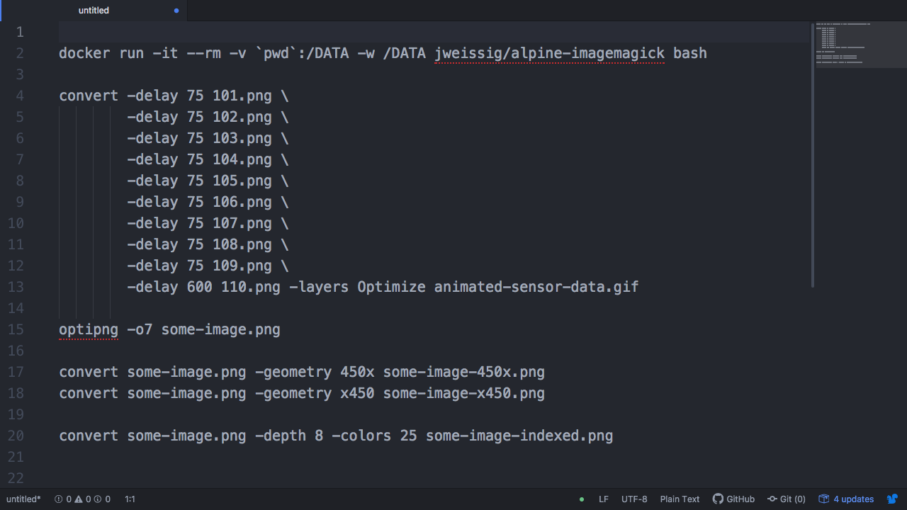
Lets jump over to an editor where I have set up a few commands. So, this first command here is the docker command that I use all the time.

What it is doing is running in interactive mode that will give us a shell, we are mounting the current directory into the container under /DATA, then setting the working directory as /DATA in the container, and finally running my Alpine ImageMagick docker image that I showed you earlier. Personally, I just find this workflow so useful as I do not have to install these tools on my laptop. I can easily move from machine to machine and this will just work. You can totally try this too.
docker run -it --rm -v `pwd`:/DATA -w /DATA jweissig/alpine-imagemagick bash
Alright, so lets copy this command and head over to the command line and run it. Great, so you can see we are in the same directory here. What I like about mounting the current directory is that changes we make in the this directory, from within the container, will persist outside the container. You know, this totally allows you to run Linux open-source tools on your Mac or Windows machines too. This is just such an awesome use-case. I am running Docker Desktop here. If you have not tried it, I highly recommend it, and it just opens so many doors.
Alright, so lets flip back to the text editor and look at the command we will use to create this animated GIF. So, I am using the convert command here, then we are asking for a 75 ms delay on this first image, same for the second, third, etc. Finally, we get to the last image and we are saying we want this one to be on the screen for 600 ms. Then it will just cycle back to the start. The output image to be saved as animated-sensor-data.gif. Lets copy this and go run it. It takes a second or two to run, but this is grabbing all of our images, and creating an animated GIF, using those time delays we asked for. Alright, so we have the image now.
convert -delay 75 101.png \
        -delay 75 102.png \
        -delay 75 103.png \
        -delay 75 104.png \
        -delay 75 105.png \
        -delay 75 106.png \
        -delay 75 107.png \
        -delay 75 108.png \
        -delay 75 109.png \
        -delay 600 110.png -layers Optimize animated-sensor-data.gif
On my desktop, outside of the Docker container, I am going to open that image. Lets flip over to it and have a look. Great, you can see it works, and we are stepping through each image, and we get a longer delay at the last image.
Lets flip back to the editor and chat about a few other commands for a minute. So, in that Alpine ImageMagick docker image, I also installed a few tools for optimizing images. You can run this optipng command to optimize png images.
optipng -o7 some-image.png
I use this heavily on the website to make it speedy. Here is some commands for resizing images, say you wanted something with a max width of 450 pixels, or maybe this one with a max height of 450 pixels.
convert some-image.png -geometry 450x some-image-450x.png
convert some-image.png -geometry x450 some-image-x450.png
Or, maybe you wanted to create an indexed image and strip out non-essential colours.
convert some-image.png -depth 8 -colors 25 some-image-indexed.png
This is sort of my swiss army knife docker image for image stuff. But, really it is more of the workflow of running utility containers like this on your local machine that I really wanted to show you. It just makes life so much easier and you do not build up all this cruft on your computer. Another really huge advantage is that you can get reproducible results and you do not need to worry about something breaking here. As, you can just use this same container over and over. Without this, I cannot tell you how many times a software upgrade, of some type, has broken tons of stuff for me, and I spend hours and hours fixing things. So, this workflow of utility containers can really save you lots of hassle as it is totally isolated and very portable.
Anyways, hopefully you will find something in here useful. That is it for this episode. Thanks for watching and I will see you next week. Bye.